import tensorflow as tf #导入tf包 import numpy as np #导入数组包 ''' 用tensorflow 实现 f(c, b) = (b+3)*(b+c) '''
'\n用tensorflow 实现 f(c, b) = (b+3)*(b+c)\n'
1 2
b = tf.Variable(2., name='b') #定义一个2.0变量为b c = tf.Variable(3., name='c') #定义一个3.0变量为c
1
2
3
4
5
#不妨设中间变量 e = (b+3) ,d = (b+c) ,a= f(b, c)吧 three = tf.constant(3., name='three') #定义一个常量3
e = tf.add(b,three) d = tf.add(b, c)
1
2
a = tf.multiply(e, d) #乘法 print(a) #结果不是25 而是一个Tensor
Tensor("Mul:0", shape=(), dtype=float32)
1 2 3 4 5 6 7 8
#真实的运行结果如下: init_top = tf.global_variables_initializer() #初始化变量 with tf.Session() as sess: #打开一个tensor会话 sess.run(init_top) #顺序不能变,先运行初始化 f = sess.run(a) #运行tensor a print(f) sess.close() #关闭会话
25.0
多组值测试
这时候我们用到tensorflow的容器
1 2
import tensorflow as tf #导入tf包 import numpy as np #导入数组包
1 2
b = tf.placeholder(tf.float32, [None, 1],name='b') #定义一个b容器,大小可以不确定,[3,1]即为3个元素,None,为未知,来源数据大小 c = tf.Variable(3., name='c') #定义一个3.0变量为c
1 2 3 4
#不妨设中间变量 e = (b+3) ,d = (b+c) ,a= f(b, c)吧
three = tf.constant(3., name='three') #定义一个常量3

e = tf.add(b,three)
d = tf.add(b, c)
1
2
a = tf.multiply(e, d) #乘法
print(a) #结果不是25 而是一个Tensor
Tensor("Mul:0", shape=(?, 1), dtype=float32)
1 2 3 4 5 6 7 8 9
#真实的运行结果如下: b_array = np.array([1,2,3,4,5]).reshape(5,1) #创建一个b的元素数组 init_top = tf.global_variables_initializer() #初始化变量 with tf.Session() as sess: #打开一个tensor会话 sess.run(init_top) #顺序不能变,先运行初始化 f = sess.run(a,feed_dict={b: b_array}) #运行tensor a, 喂食词典 b的元素 来源于 b_array print(f) #输出必然是多组值 sess.close() #关闭会话
[[16.]
[25.]
[36.]
[49.]
[64.]]
好了函数介绍就到这
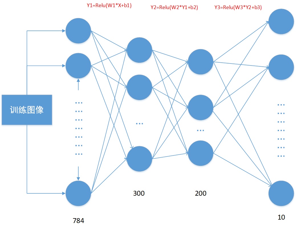
MNIST 手写字体训练
注释解释的很清楚,推荐有基础的人去看,新手会完全看不懂的
1 2 3 4 5 6 7 8 9
import tensorflow as tf from tensorflow.examples.tutorials.mnist import input_data import numpy as np import matplotlib.pyplot as plt